Direct model calibration on a fault using Map3Di

Direct model calibration on a fault using Map3Di

For a fault slip calibration one would define the location of the structure from intersections, seismicity and geological interpretation (as before), then integrate the effect of the seismicity associated with the fault to determine the distribution of slip on the fault surface. This slip is then applied in Map3Di as a prescribed non-homogeneous shear discontinuity. The slip is accumulated as seismicity occurs and used to further load the model.

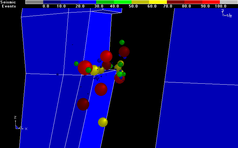
As a demonstration of how the Map3Di analysis would proceed, consider the example shown below. The location of a fault structure has been defined and is shown with the seismicity.

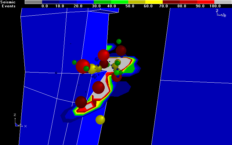
The seismicity associated with the fault is then integrated to determine the distribution of slip on the fault surface that is implyed.

This slip is then applied directly into the Map3Di numerical model as a prescribed non-homogeneous shear discontinuity. A stress analysis can now be conducted to simulate the interaction between the slip implied by the seismicity and the stoping (and any other features incorporated into the model, e.g. slipping faults, dykes etc.). Below, a model has been run without modelling the fault (the fault could also be modelled if desired), but including slip implied by the seismicity. In this figure, the excess shear stress at the location of the fault surface is presented (using a 20° friction angle).

|t| - Sn tan(j)

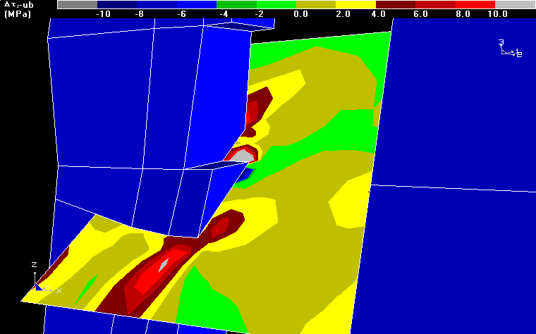
The results show that over most of the fault surface, there is little or no excess shear stress and hence no further potential for slip at these locations (although additional slip could be induced if other parts of the fault were to slip). However at a few locations (to the front and right of the left most stope) there is still considerable excess shear stress. This could indicate that the fault is hung up at these locations. Alternatively, this may simply be a result of improperly distributing the slip over the fault plane. In either case, there is considerable potential for slip yet the seismicity has not indicated that this has occurred. Part of the value in applying this procedure is to identify such areas. Further study of this location (including a detailed review of the seismicity and perhaps an in situ investigation) is certainly warranted.

Note that by applying this procedure we have bypassed the trial and error back-analysis stage and thus reduced the amount of engineering effort required to calibrate our model. Once the prescribed shear discontinuity is applied we have by definition a model that matches previously observed behaviour, and we are in a better position to make forward predictions.

This goes along way towards satisfying our first calibration objective: to bring the model to a state most representative of the currently observed conditions. By calibrating our numerical model using seismic loading we can actually bring the model into an initial state much closer to in situ conditions then we could ever hope to achieve by the trial and error approach. Non-uniform slip distributions over a fault surface, derived from the observed seismicity, have been directly imposed into the numerical model. The amount of trial and error that would be required to determine this shear strength distribution would be formidable.

We can now take this procedure one step further. We can use these results as a direct back-analysis method. This would proceed by subdividing the fault into small elements and back-calculating the shear strength in each element that is required to bring about the specified slip

j = tan-1 (|t| / sn)

This is illustrated below where the friction angle distribution necessary to resist slip is presented.

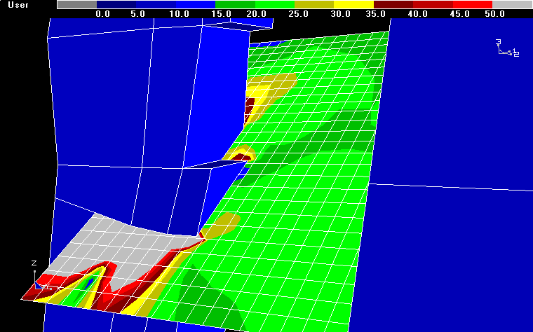
The results show that over most of the fault surface, a nearly constant friction angle of approximately 20° is required. However in front of the left most stope a very high value is required to resist slip. This suggests that the fault has hung up at this location. It is possible that an asperity due to some local bend, wave or offset in the fault is responsible for this. Additional in situ investigation would be advised to verify this.

We are now in a position to build a non-linear fault model with this heterogeneous shear strength distribution. Such a model would deform to match the slip distribution observed from the seismicity. We now have a model that not only matches previously observed behaviour, but is also calibrated with the exact strength distribution required to evolve to this known state. This does two things for us: it gives us a calibrated model to make forward predictions with, and through repeated back-analyses allows us to test how well our model matches previously observed behaviour.

This goes along way towards satisfying both of our calibration objectives: to bring the model to a state most representative of the currently observed conditions, and characterization of geological features. It is clear that the resulting model is far better calibrated to observed in situ conditions than one could ever hope to achieve by using a best-fit homogeneous strength assumption. A homogeneous strength assumption would not allow for simulation of the observed asperity.

It must be emphasized that this procedure constitutes identification of flaws in the rockmass. In this case, microseismic activity is not only being used to identify the presence of these flaws, but also characterize the behaviour and impose the effect implied by the seismicity into the model. This technique provides a unique opportunity for construction of mine wide stability models incorporating major structural features.

1. Unzip smn.zip to create smn.001 and smn.ms.
2. To display these results in Map3D, use File > Open Analysis Results and select smn.001.
3. To load the seismic events, use the Visualization function and specify the user file and smn.ms.
4. To display the seismic events, clicking the Plot button.
5. These can be contoured by checking Contoured Colours, then clicking the Plot button.
6. These can be scaled to the magnitude by checking Scaled Radius, then clicking the Plot button.
7. A plane can be fitted through the data by selecting Plane > Linear Regression, then selecting Sum in Voxel.